Workflows
Table of contents
- Conformational Search Algorithms
- Protonation Site Screening
- Automated Reaction Discovery for Mass Spectra Elucidation (MSREACT)
- Quantum Cluster Growth (QCG)
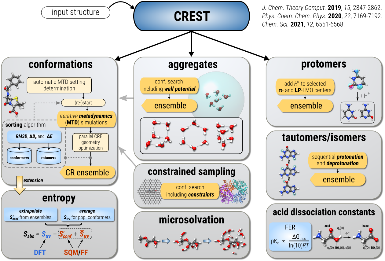
Conformational Search Algorithms
iMTD-GC Algorithm
For detailed information see Phys. Chem. Chem. Phys., 2020, 22, 7169-7192.
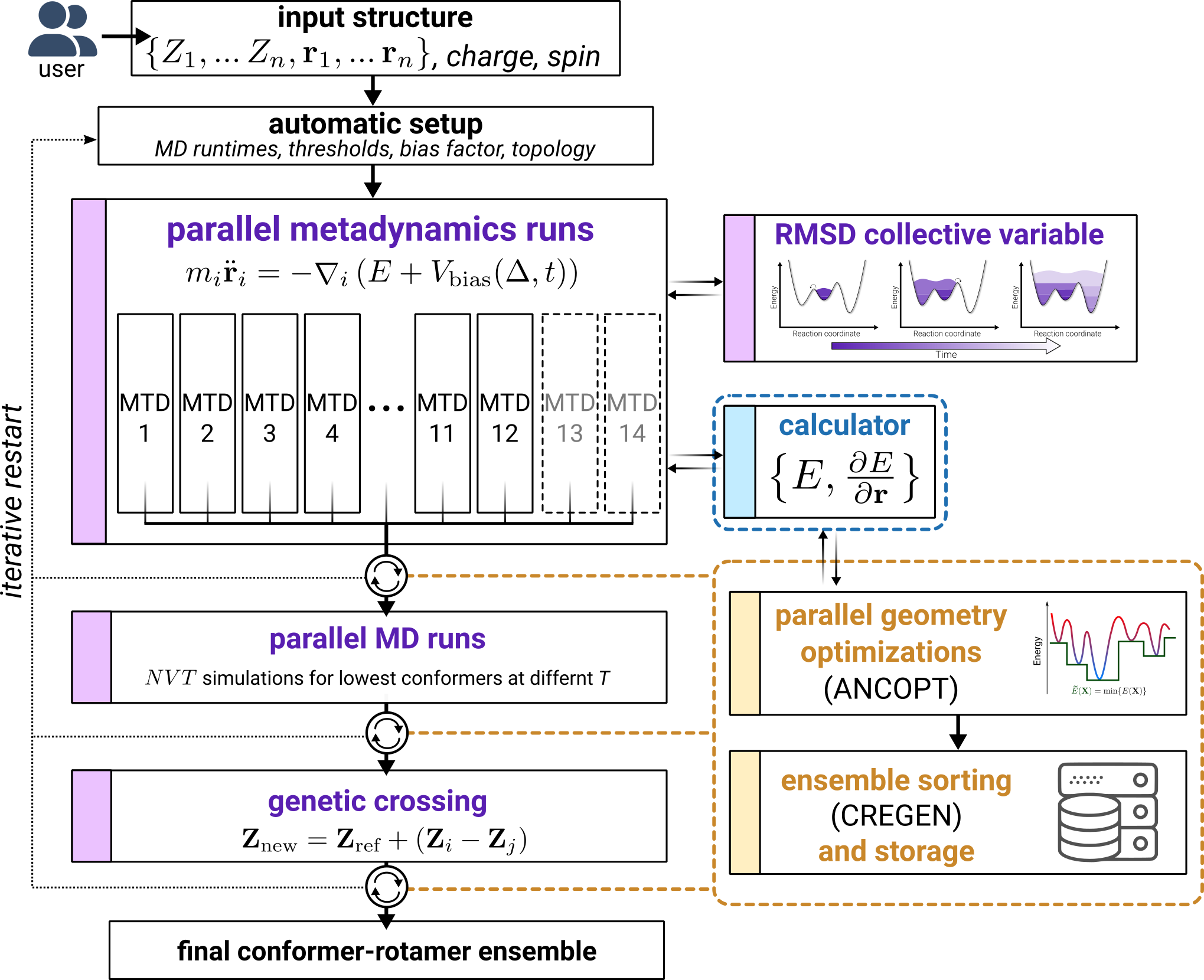
The iMTD-GC workflow was designed to find low lying conformers more efficiently and more safely than the older MF-MD-GC algorithm (discontinued algorithm in the original version of CREST). Furthermore this new algorithm is more robust and generally applicable than more complicated schemes since it does not require any pre-definition of special system coordinates. iMTD-GC is rooted in the basic idea to combine GFNn-xTB calculations with root-mean-square-deviation (RMSD) based metadynamics simulations. In practice, a history-dependent biasing potential is applied, where the collective variables (CVs) for the metadynamics are previous minima on the PES, expressed as RMSD between the structures. The biasing contribution is given by Gaussian-type potential as
\(V_\text{bias} = \sum^n_i k_i \exp ( -\alpha \Delta_i^2)~,\)
where the RMSD enter as collective variables \(\Delta_i\), n is the number of reference structures, ki are the pushing strengths and the parameter \(\alpha\) determines the potentials’ shape. From this energy expression atomic forces are derived that enter as additional forces in the MTD simulations (in the context of meta-dynamics also sometimes refered to as guiding forces). The MTD procedure can be though of as an energy penalty for the current MD snapshot, should it be too similar to one or more previously documented reference structures. Continously updating the reference structure list, over time,allows otherwise unlikely high-barrier crossings where all atoms collectively explore huge regions of the potential energy surface.
Genetic Z-matrix crossing (GC) is related to the concept of genetic algorithms in such that structural elements present only in already generated structures are projected onto a reference to create new structures. By repeating the crossing procedures structural elements that appear more frequently would be inherited more often, being responsible for the ‘genetic’ character of this approach. Internal (Z-matrix, R) coordinates are employed and a new structure is generated by taking the differences to the reference Rref over all internal coordinates (i.e., bond length, bond angles, an dihedral angles) according to
\(R_\text{new} = R_\text{ref} + R_{i} - R_{j}~,\)
where Ri and Rj label the pairs and Rnew is the generated new structure, which is subjected to a full geometry optimization. In this way, structural differences, e.g. a methyl group rotation, relative to Rref present only in Ri and Rj are combined in the resulting new conformer/rotamer. The ensemble can be improved regarding the rotamers efficiently by the Z-matrix crossing. This effect is best visible for acyclic chains with a number of rotateable bonds, e.g., alkanes, but in principle it also works for more complicated cases, such as macrocyclic systems.
In practice, the MTD simulation length is determined automatically by a flexibility measure of the molecule (typically \(t = 0.3-0.4 \times N\) ps per MTD). Several independent MTDs (at 300 K) are performed with different setings for \(\alpha\) (in Bohr-1) and ki/N (in mEh). This has to be done since each molecule in principle requires a unique set of optimal \(\alpha\) and k and thus a variety of parameters ensures that the algorithm is perfroming well for all types of molecules. The snapshots are geometry optimized in a multi-level, three-step-filtering procedure by firstly applying two loose threshold settings followed by very tightly converged optimization and energy windows of 15, 10, and 6 kcal/mol, respectively. After the second step of this filtering, some short regular MD simulations are performed on the 6 lowermost conformers (at different temperatures 400 and 500 K), which is done to A) get rotamers and B) more extensively sample around these minima on the PSE (i.e., find low-barrier conformers missed by the high-energy MTD treatment). In the last step the GC procedure is performed to further complete the CRE. The number of generated structures in this step is limited to \(\text{min}(3000,t\times 50)\) in order to limit the computational cost. Furthermore a two-step-filtering procedure is used to optimize the generated geometries, similar to the three-step-filtering before.
The algorithm is iterative, i.e., if a new lower conformer is found at any point during the sampling the procedure is restarted with this conformer as an input. All CREs that are found within the iterations are included in the conformer/rotamer ranking process. The iMTD-GC worflow is outlined graphically in the figure below.
Conformational Entropy Calculations
For detailed information see Chem. Sci., 2021, 12, 6551-6568.
Following CREST version 2.11, a new variant of the iMTD-GC workflow is introduced called iMTD-sMTD. The important new part of this algorithm are so-called static metadynamics simulations (sMTD), which are practically more similar to umbrella sampling or basing-hopping algorithms. Here, in each sMTD, previously found conformers are added via Vbias as a global potential and, opposed to the iMTD workflow, are not updated with new structures during the simulation. Several iterations of sMTD are executed until convergence is achived with regards to the ensemble entropy and number of conformers in the ensemble. After each sMTD iteration, new bias structures for the potential are identified via an PCA and k-Means ensemble clustering approach with dihedral angles as descriptors. The iMTD-sMTD workflow is outlined in the figure below.
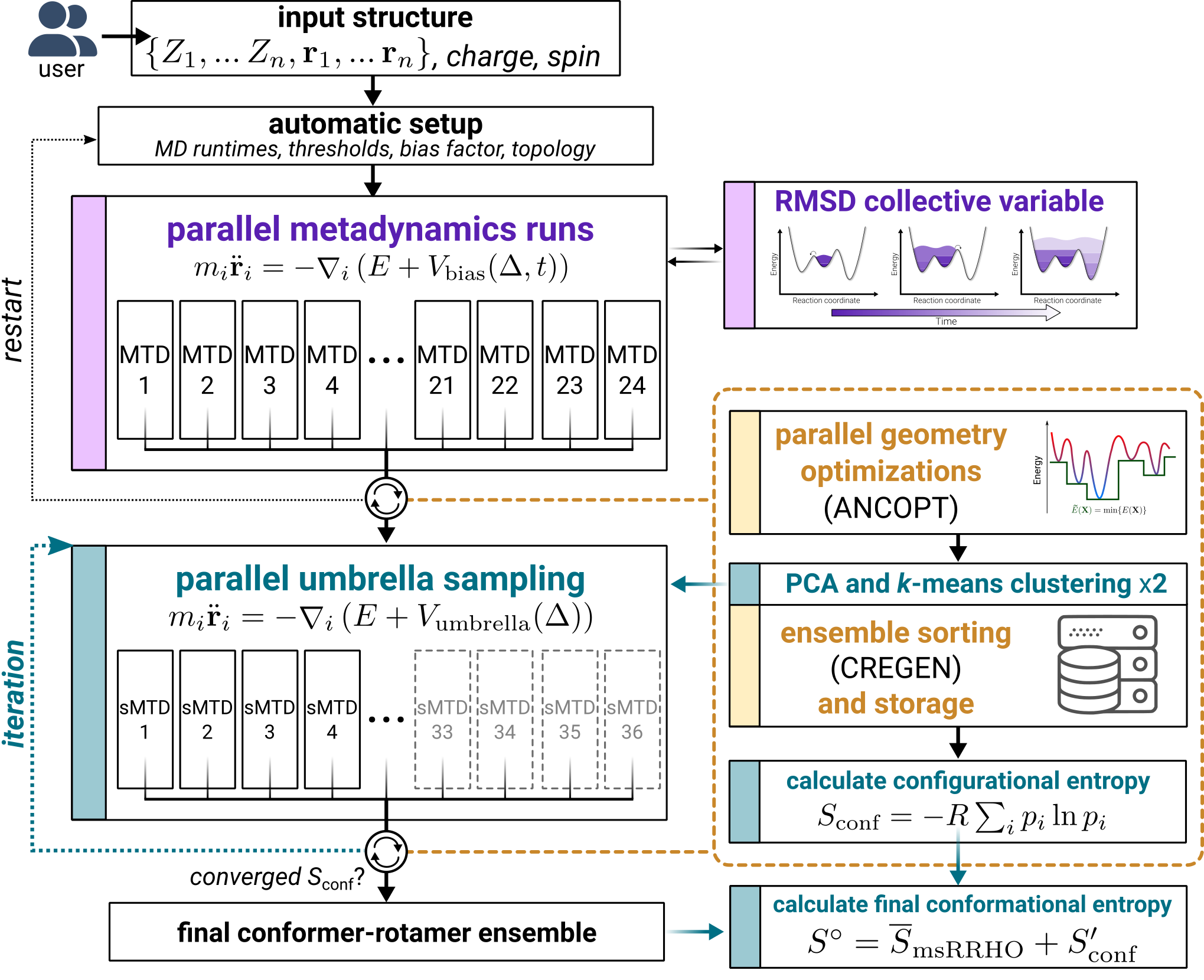
This algorithm can be used not only for ensemble generation, but also provides the capability to determine a converged conformational entropy. After convergence this requires only two additional steps (outlined as the gray boxes in the figure), which are an extrapolation of the entropy based on the iterations of sMTD-iMTD and an averaged thermostatistical contribution \(\overline{S}_\text{msRRHO}\).
--v4 or for entropy calculations with the keyword --entropyConstrained Conformational Sampling
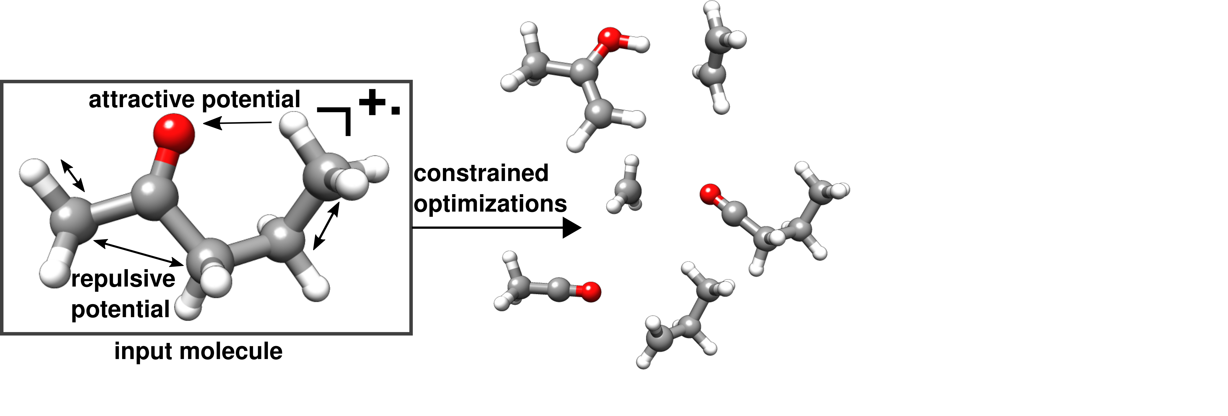
For some systems constraints have to be introduced. This can be the case, for example, if a non-covalently bound complex shall be investigated. Here, the metadynamics bias would simply push the aggregated molecules apart since this maximizes the RMSD (and minimizes the respective MTD energy penalty). In other cases, some bond could be not well described by the unerlying SQMSemiempirical Quantum Mechanics. On this site, SQM usually refers to the GFNn-xTB methods. method and needs to be constrained. Luckily, those cases can be easily treated within the metadynamics framework. Basically all CREST workflows allow the introduction of various geometrical constraints into the calculations. An examle is shown [here][].
Protonation Site Screening
For detailed information see J. Comput. Chem. 2017, 38 (30), 2618-2631.
One of the initial screening applications of GFN-xTB is the identification and ranking of protonation sites. The procedure is fairly straight-foward as it involves only the generation of protonated starting geometries, which are then simply optimized and ranked according to their total energies. Centers for the protonation are determined from the electronic structure at the tight-binding level. The respective molecular orbitals are localized and π- and LP-centers are identified. To each of these centers a proton is added to generate a corresponding starting geometry, which is then optimized with the molecular charge increased by one. The procedure is outlined in the figure below for the example of benzocaine.
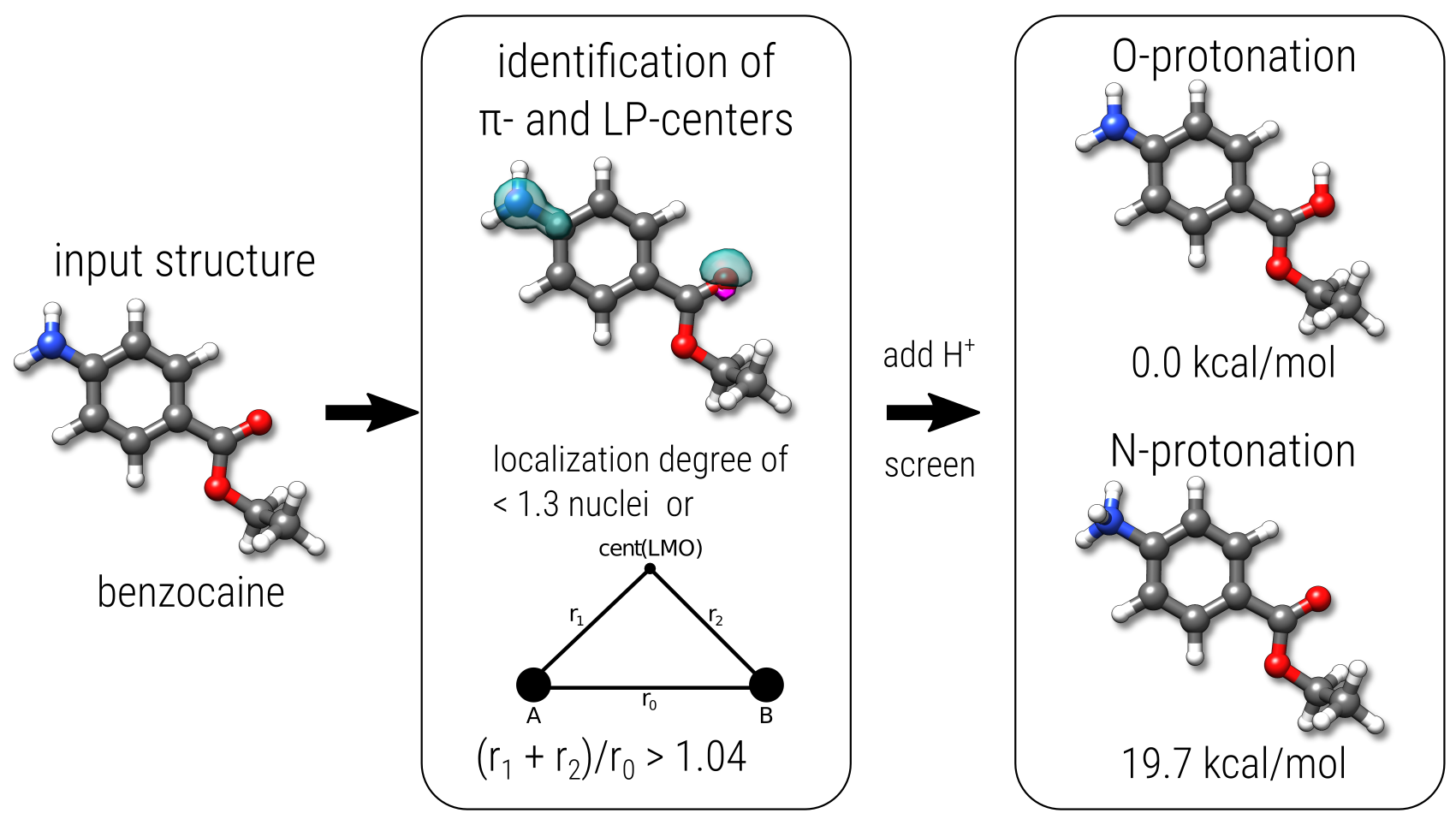
As a variation of this procedure, also the screening of deprotonation sites is possible. Here, no quantumchemical information (orbitals) is required. Instead, starting points are generated by simply removing hydrogen atoms from the initial (neutral) structure. The generated structures are then optimized under the constraint of a molecular charge decreased by one.
Conducting a sequence of protonation and deprotonation screening steps can be used as a sampling procedure for protortopic tautomers, which is also implemented.
Automated Reaction Discovery for Mass Spectra Elucidation (MSREACT)
For detailed information see [J. Chem. Phys., 2024, submitted.]{}
The MSREACT tool of CREST aids reaction exploration with a special focus on creating fragments and rearrangement products (isomers) occurring in mass spectrometry (MS) experiments, such as electron ionization (EI) or Electrospray Ionization/Collision In- duced Dissociation (CID/ESI). Systematic generation of possible products for the input molecule is achieved through the application of constraining potentials between atom pairs and optimization using an efficient SQM method. Interatomic distances are deliberately extended well beyond their equilibrium values, inducing dissociation and rearrangement re- action products.
Go to the MSREACT keyword documentation
Quantum Cluster Growth (QCG)
For detailed information see J. Chem. Theory Comput., 2022, 18 (5), 3174-3189.
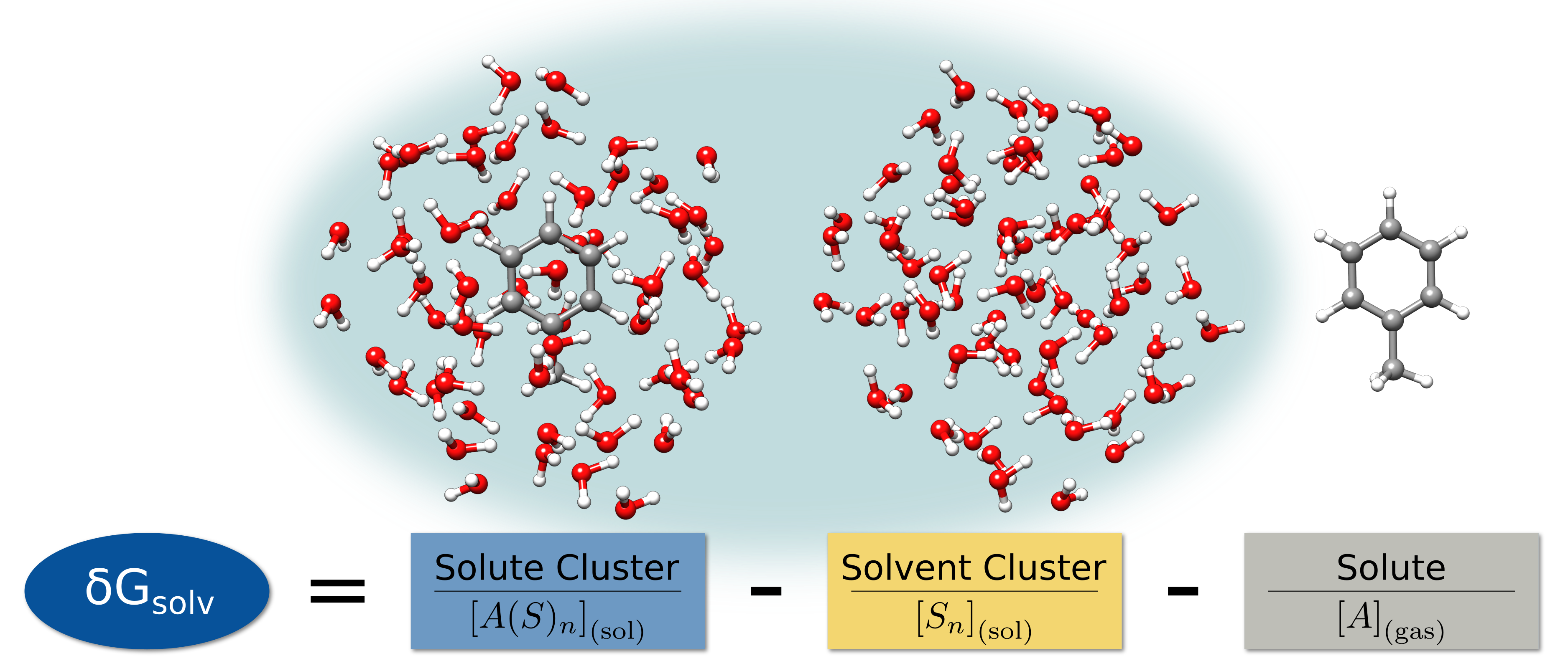
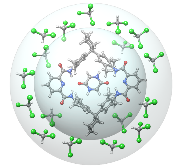
Quantum Cluster Growth is a utility/driver extension of CREST for the xtb program. It is designed to automatically add explicit solvent molecules to a solute, to generate an ensemble of the resulting cluster, and to compute solvation free energies in an explicit fashion. Thereby, almost any solute–solvent combination can be used, including open-shell and charged solutes.
The key procedure is the automated addition of solvent molecules around the solute, mainly done by a screening of docking positions, using the aISS docking algorithm or the xtbiff program, and xtb geometry optimizations. A second step includes the ensemble generation, which can be done either with single a MD/MTD simulation or the NCI-MTD workflow of CREST. The solvation free energy can additionally be computed by generating a reference ensemble.
Go to the QCG keyword documentation
Automated Grow Algorithm and Ensemble Generation
The automated grow algorithm starts with input coordinates provided by the user. Also, additional information like the charge and the number of unpaired electrons of the solute can be given, as well as the number of solvent molecules that should be added. As performing an unbiased docking of the solvent would lead to solvent clustering, two wall potentials are applied.
The inner one causes the solute to stay in the center, while the outer one prevents the solvent molecules from clustering and causes the solvent to surround the solute. Having the prerequisites set, first an aISS (or xtbiff) docking of a solute and solvent molecule is performed under application of the wall potentials. Second, a geometry optimization is done with xtb. These two steps repeat until the user-defined number of solvents is added.
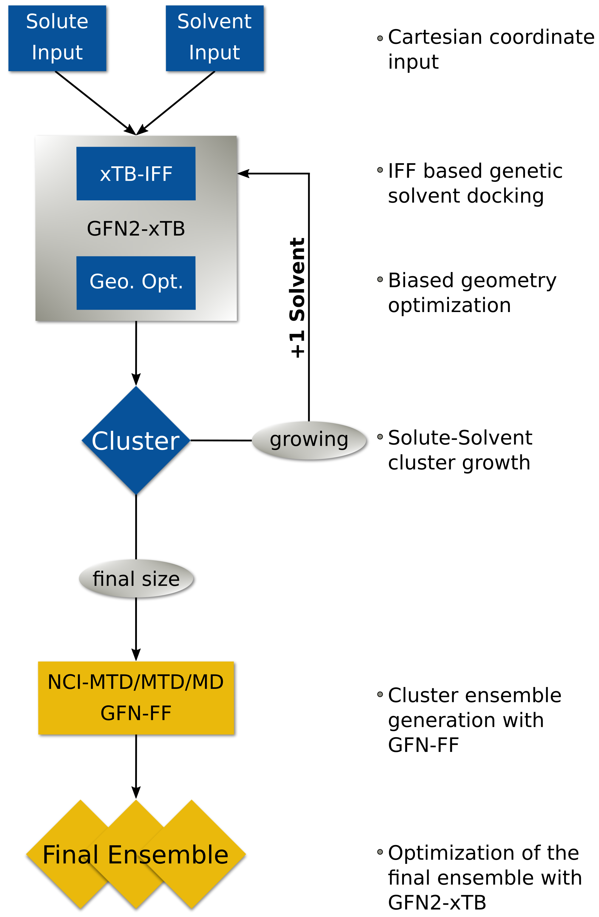
The ensemble generation will also be performed with the wall potentials. It can be done with just an MD or MTD simulation and optimizing the snapshot geometries. Anyway, the NCI-MTD run-type is recommended and set as default because it explores the conformational space the most. It can be further enhanced by increasing the MTD time during this run-type or by decreasing the sampling frequency of snapshots.
Solvation Free Energy
The solvation free energy can also be computed with QCG in a supermolecular approach. To do so, a reference ensemble has to be generated first. By default, this is done with the Cut-Freeze-Fill (CFF) algorithm. It removes the solute from the highest populated clusters of the solute–solvent ensemble and fills the remaining cavity with solvents. Afterward, frequency calculations are performed for the solute–solvent and the reference ensembles, as well as the solute. These give rise to thermocorrections. After scaling the translational and rotational entropy and taking the conformational entropy into account, the free energies are obtained. Substracting the free energy of the reference ensemble and the solute from the solute–solvent ensemble, yields finally the solvation free energy.