QCG Example 3

An example for constrained QCG calculations.

Constraining the solute

Sometimes GFN2-xTB or GFN-FF geometry optimizations might distort DFT optimized structures. To prevent this, it is possible to constrain the solute geometry by adding a file .xcontrol with constraints to the calculation. A typical example where this is necessary are transition metal molecules, such as the iron complex below.

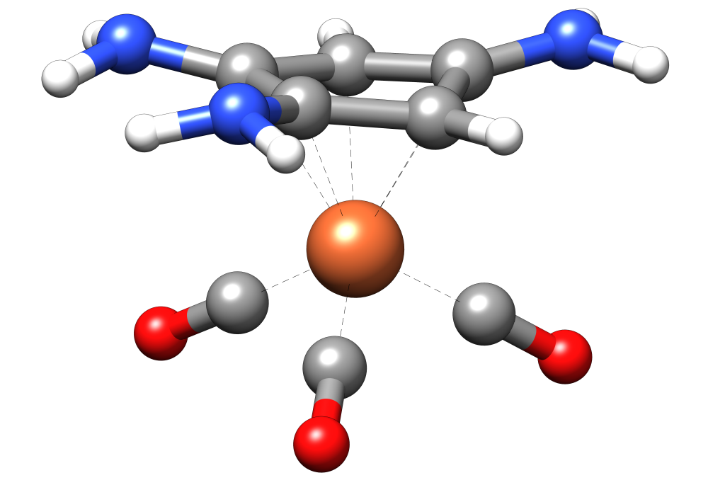
Fe-complex — DFT optimized structure of an Fe(II)-complex

Warning: Contrary to other CREST applications, constraining the structure in QCG requires the constraining file to be named .xcontrol. The file is read automatically by the QCG procedure and can’t be specified separately via the command line.

Now we want to constrain the ligands and to generate an ensemble. To do so, we provide the following .xcontrol file that constrains all bonds between the iron (16), the carbon atoms of the ring (atoms 3,4,6,7,8), and the CO ligands (atoms 17-22):

$constrain
  atoms: 3,4,6-8,16,17-22
$end

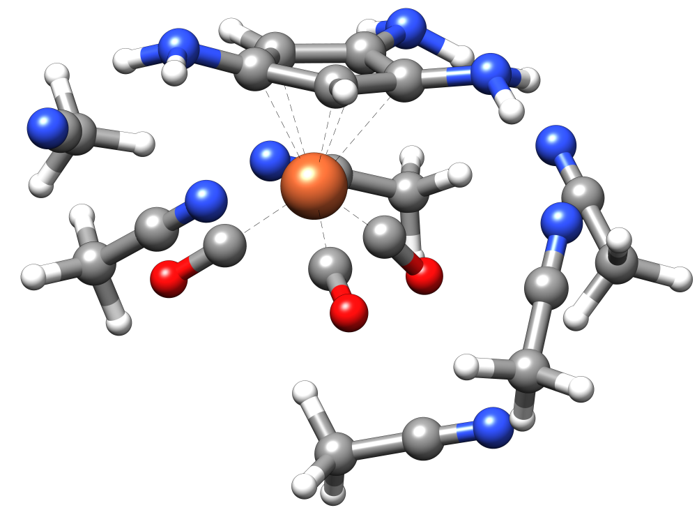
Having prepared a directory with this file named .xcontrol, the solute coordinates solute.xyz, and the solvent coordinates solvent.xyz (acetonitrile), the ensemble is now generated for example with

crest solute.xyz --qcg solvent.xyz --nsolv 6 --T 12 --ensemble --gbsa h2o --mdtime 50 --mddump 200

 23

N          1.3802608000       -0.0318528000        0.0463356000
N         -0.4099459000       -2.4279732000       -0.4426793000
C         -0.8233287000       -1.1730691000       -0.1562094000
C          0.0282237000       -0.0329935000        0.0761397000
N         -3.1128965000        1.1237167000        1.4357707000
C         -0.8148438000        1.0531548000        0.5128170000
C         -2.1758731000       -0.7690355000        0.1411386000
C         -2.1257237000        0.5229799000        0.7675646000
H         -0.4572325000        2.0269118000        0.8223111000
H         -4.0464379000        0.7439366000        1.3737637000
H         -3.0303702000        2.1068597000        1.6506659000
H         -1.1169391000       -3.0848452000       -0.7424315000
H          0.4822106000       -2.5429436000       -0.9026828000
H          1.8456312000       -0.7155480000       -0.5345244000
H          1.8360609000        0.8698550000        0.0667192000
H         -3.0359762000       -1.4262449000        0.1182750000
Fe        -1.5405186000        0.5270943000       -1.3978036000
C         -1.8580173000       -0.6232521000       -2.7083661000
C         -2.9303295000        1.6215990000       -1.6740517000
C         -0.3124958000        1.4435812000       -2.2886848000
O          0.5082387000        2.0393586000       -2.8321404000
O         -2.0651590000       -1.4011695000       -3.5304385000
O         -3.8189784000        2.3247399000       -1.8686288000

  6

C         -5.1936370000        1.8144547000       -0.0000255000
C         -3.7637653000        1.6301290000       -0.0000193000
H         -5.5336302000        2.0849167000        0.9967301000
H         -5.6871686000        0.8944148000       -0.3037251000
H         -5.4665453000        2.6066235000       -0.6930206000
N         -2.6155337000        1.4820613000        0.0000603000

Two ensembles will result:

a “complete” one named full_ensemble.xyz
and one with only the highest populated clusters final_ensemble.xyz)

All ensembles will have a solute structure that has the same Fe-C geometries as the solute.xyz file.

Fe-complex with acetonitrile — A selected structure of the (micro)solvated iron complex from the ensemble.

Important: If the solute is constrained completely, the preoptimization of the solute will fail. Therefore, the preoptimization should be switched off with --nopreopt.